Definition
We’ll start by defining the Kullback–Leibler (KL) divergence. It is defined as: $$D_{K L}(P(x) | Q(x))=\sum_{i=1}^B P\left(x_i\right) \cdot \ln \left(\frac{P\left(x_i\right)}{Q\left(x_i\right)}\right)$$
where (P) is the original distribution and (Q) is the current distribution.
The KL divergence measures how one, actual probability distribution diverges from a second, expected probability distribution. $B$ is defined as the number of bins in the histogram, which in our application would be the the number of unique values in the distributions.
Implementation
The PySpark code is an altered version of the Scala implementation by Albertus Kelvin.
import pyspark.sql.functions as F
import pyspark.sql as ps


class KLDivergenceColumns:
    """Columns used in KL Divergence calculations."""

    DSHIFT_KLDIV_SAMPLE_FREQUENCY = "sample_frequency"
    DSHIFT_KLDIV_ORIGIN_PROBA_DISTR = "origin_proba_distr"
    DSHIFT_KLDIV_CURRENT_PROBA_DISTR = "current_proba_distr"
    DSHIFT_KLDIV_STATISTIC = "kl_div_statistic"


def calculate_kullback_leibler_divergence(
    df_origin: ps.DataFrame,
    df_current: ps.DataFrame,
    column: str,
) -> float:
    """Calculates the Kullback-Leibler divergence for a given column."""
    df_origin_sample_count = df_origin.groupBy(column).agg(
        F.count("*").alias(KLDivergenceColumns.DSHIFT_KLDIV_SAMPLE_FREQUENCY)
    )

    df_current_sample_count = df_current.groupBy(column).agg(
        F.count("*").alias(KLDivergenceColumns.DSHIFT_KLDIV_SAMPLE_FREQUENCY)
    )

    # Apply smoothing
    smoothed_origin = smooth_distribution_sample(
        df_origin_sample_count, df_current_sample_count, column
    )
    smoothed_current = smooth_distribution_sample(
        df_current_sample_count, df_origin_sample_count, column
    )

    # Calculate probability distributions
    origin_proba = compute_proba_distribution_from_freq_counts(
        smoothed_origin, KLDivergenceColumns.DSHIFT_KLDIV_ORIGIN_PROBA_DISTR
    )

    current_proba = compute_proba_distribution_from_freq_counts(
        smoothed_current, KLDivergenceColumns.DSHIFT_KLDIV_CURRENT_PROBA_DISTR
    )

    # Calculate KL divergence
    kl_div = compute_kl_div_statistic(origin_proba, current_proba, column)

    return kl_div


def smooth_distribution_sample(
    df_target: ps.DataFrame, df_complement: ps.DataFrame, column: str
) -> ps.DataFrame:
    """
    Creates a smoothed sample by handling unobserved values in the target DataFrame.

    Args:
        df_target: The target distribution DataFrame with [EventType, Count]
        df_complement: The complement distribution DataFrame with potential new values

    Returns:
        DataFrame with smoothed distribution
    """
    # Find unobserved target samples
    df_unobserved_target_sample = df_complement.join(
        other=df_target, on=column, how="left_anti"
    ).distinct()

    # Assign frequency to unobserved samples
    unobserved_target_sample_count_df = df_unobserved_target_sample.withColumn(
        KLDivergenceColumns.DSHIFT_KLDIV_SAMPLE_FREQUENCY, F.lit(0.0001)
    )

    # Combine observed and unobserved samples
    columns = df_target.columns
    return unobserved_target_sample_count_df.select(*columns).union(df_target)


def compute_proba_distribution_from_freq_counts(
    df: ps.DataFrame, proba_distr_col_name: str
) -> ps.DataFrame:
    """
    Computes probability distribution from frequency counts.

    Args:
        df: DataFrame with frequency counts
        proba_distr_col_name: Column name for the probability distribution

    Returns:
        DataFrame with probability distribution
    """
    # Calculate total observations
    row_total_observations = df.agg(
        F.sum(F.col(KLDivergenceColumns.DSHIFT_KLDIV_SAMPLE_FREQUENCY))
    ).first()

    if row_total_observations is None:
        raise ValueError("Total observations calculation resulted in None.")

    total_observations = row_total_observations[0]

    # Calculate probability distribution
    return df.withColumn(
        proba_distr_col_name,
        F.col(KLDivergenceColumns.DSHIFT_KLDIV_SAMPLE_FREQUENCY)
        / F.lit(total_observations),
    ).drop(KLDivergenceColumns.DSHIFT_KLDIV_SAMPLE_FREQUENCY)


def compute_kl_div_statistic(
    origin_sample_proba_distr_df: ps.DataFrame,
    current_sample_proba_distr_df: ps.DataFrame,
    column: str,
) -> float:
    """
    Computes the KL divergence statistic between two probability distributions.

    Args:
        origin_sample_proba_distr_df: DataFrame with origin probability distribution
        current_sample_proba_distr_df: DataFrame with current probability distribution

    Returns:
        KL divergence statistic
    """
    # Join probability distributions
    df_pair_of_proba_distr = origin_sample_proba_distr_df.join(
        other=current_sample_proba_distr_df,
        on=column,
        how="inner",
    )

    # Calculate KL divergence
    df_pair_of_proba_distr = df_pair_of_proba_distr.withColumn(
        KLDivergenceColumns.DSHIFT_KLDIV_STATISTIC,
        F.col(KLDivergenceColumns.DSHIFT_KLDIV_ORIGIN_PROBA_DISTR)
        * F.log(
            F.col(KLDivergenceColumns.DSHIFT_KLDIV_ORIGIN_PROBA_DISTR)
            / F.col(KLDivergenceColumns.DSHIFT_KLDIV_CURRENT_PROBA_DISTR)
        ),
    )

    df_pair_of_proba_distr = df_pair_of_proba_distr.drop(
        KLDivergenceColumns.DSHIFT_KLDIV_ORIGIN_PROBA_DISTR,
        KLDivergenceColumns.DSHIFT_KLDIV_CURRENT_PROBA_DISTR,
    )

    kl_divergence = df_pair_of_proba_distr.agg(
        F.sum(F.col(KLDivergenceColumns.DSHIFT_KLDIV_STATISTIC))
    ).first()

    if kl_divergence is None:
        raise ValueError("KL Divergence calculation resulted in None.")

    return kl_divergence[0]
Example usage
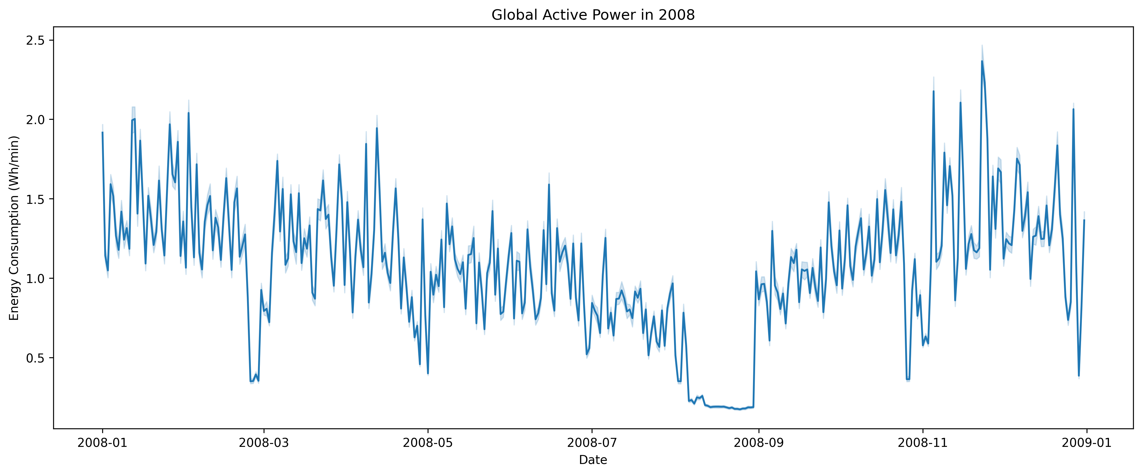
I’ll use the Individual household electric power consumption dataset from UCI ML Repository as an example for how to use the Kullback-Liebler metric for data drift detection.
We want to monitor data drift in the column "Global_active_power".
We’ll set up a local PySpark session. Normally you would run this on a cluster, e.g. on Databricks, but for this example, we’ll run it locally.
spark = (
    SparkSession.builder.appName("Data Drift")
    .config("spark.sql.execution.arrow.pyspark.enabled", "true")
    .config("spark.sql.execution.arrow.pyspark.fallback.enabled", "true")
    # Set partitions to a lower number than the default 200
    # as we're working with a small dataset
    .config("spark.sql.shuffle.partitions", "10")
).getOrCreate()

df = (
    spark.read.option("delimiter", ";")
    .options(header=True)
    .csv(
        "./household_power_consumption.txt"
    )
)
We’lll have to do some preprocessing before continuing as we need to construct a datetime column from the Date and Time columns, as well as convert the columns to the correct types.
def preprocess_data(df: ps.DataFrame) -> ps.DataFrame:
    df = df.select(
        F.to_date("Date", format="d/M/yyyy").alias("Date"),
        F.col("Time"),
        F.col("Global_active_power").cast("double"),
        F.col("Global_reactive_power").cast("double"),
        F.col("Voltage").cast("double"),
        F.col("Global_intensity").cast("double"),
        F.col("Sub_metering_1").cast("double"),
        F.col("Sub_metering_2").cast("double"),
        F.col("Sub_metering_3").cast("double"),
    )

    df = df.withColumn(
        "DateTime",
        F.to_timestamp(
            F.concat(F.col("Date"), F.lit(" "), F.col("Time")), "yyyy-M-dd HH:mm:ss"
        ),
    )
    # Nearest hour
    df = df.withColumn("DateTimeHour", F.date_trunc("hour", F.col("DateTime")))
    df = df.withColumn("Date", F.col("DateTime").cast("date"))

    df = df.drop("Time")
    return df

df = preprocess_data(df)
df.show()
>
+----------+-------------------+---------------------+-------+----------------+--------------+--------------+--------------+-------------------+-------------------+
|      Date|Global_active_power|Global_reactive_power|Voltage|Global_intensity|Sub_metering_1|Sub_metering_2|Sub_metering_3|           DateTime|       DateTimeHour|
+----------+-------------------+---------------------+-------+----------------+--------------+--------------+--------------+-------------------+-------------------+
|2006-12-16|              4.216|                0.418| 234.84|            18.4|           0.0|           1.0|          17.0|2006-12-16 17:24:00|2006-12-16 17:00:00|
|2006-12-16|               5.36|                0.436| 233.63|            23.0|           0.0|           1.0|          16.0|2006-12-16 17:25:00|2006-12-16 17:00:00|
|2006-12-16|              5.374|                0.498| 233.29|            23.0|           0.0|           2.0|          17.0|2006-12-16 17:26:00|2006-12-16 17:00:00|
|2006-12-16|              5.388|                0.502| 233.74|            23.0|           0.0|           1.0|          17.0|2006-12-16 17:27:00|2006-12-16 17:00:00|
|2006-12-16|              3.666|                0.528| 235.68|            15.8|           0.0|           1.0|          17.0|2006-12-16 17:28:00|2006-12-16 17:00:00|
|2006-12-16|               3.52|                0.522| 235.02|            15.0|           0.0|           2.0|          17.0|2006-12-16 17:29:00|2006-12-16 17:00:00|
|2006-12-16|              3.702|                 0.52| 235.09|            15.8|           0.0|           1.0|          17.0|2006-12-16 17:30:00|2006-12-16 17:00:00|
|2006-12-16|                3.7|                 0.52| 235.22|            15.8|           0.0|           1.0|          17.0|2006-12-16 17:31:00|2006-12-16 17:00:00|
|2006-12-16|              3.668|                 0.51| 233.99|            15.8|           0.0|           1.0|          17.0|2006-12-16 17:32:00|2006-12-16 17:00:00|
|2006-12-16|              3.662|                 0.51| 233.86|            15.8|           0.0|           2.0|          16.0|2006-12-16 17:33:00|2006-12-16 17:00:00|
|2006-12-16|              4.448|                0.498| 232.86|            19.6|           0.0|           1.0|          17.0|2006-12-16 17:34:00|2006-12-16 17:00:00|
|2006-12-16|              5.412|                 0.47| 232.78|            23.2|           0.0|           1.0|          17.0|2006-12-16 17:35:00|2006-12-16 17:00:00|
|2006-12-16|              5.224|                0.478| 232.99|            22.4|           0.0|           1.0|          16.0|2006-12-16 17:36:00|2006-12-16 17:00:00|
|2006-12-16|              5.268|                0.398| 232.91|            22.6|           0.0|           2.0|          17.0|2006-12-16 17:37:00|2006-12-16 17:00:00|
|2006-12-16|              4.054|                0.422| 235.24|            17.6|           0.0|           1.0|          17.0|2006-12-16 17:38:00|2006-12-16 17:00:00|
|2006-12-16|              3.384|                0.282| 237.14|            14.2|           0.0|           0.0|          17.0|2006-12-16 17:39:00|2006-12-16 17:00:00|
|2006-12-16|               3.27|                0.152| 236.73|            13.8|           0.0|           0.0|          17.0|2006-12-16 17:40:00|2006-12-16 17:00:00|
|2006-12-16|               3.43|                0.156| 237.06|            14.4|           0.0|           0.0|          17.0|2006-12-16 17:41:00|2006-12-16 17:00:00|
|2006-12-16|              3.266|                  0.0| 237.13|            13.8|           0.0|           0.0|          18.0|2006-12-16 17:42:00|2006-12-16 17:00:00|
|2006-12-16|              3.728|                  0.0| 235.84|            16.4|           0.0|           0.0|          17.0|2006-12-16 17:43:00|2006-12-16 17:00:00|
+----------+-------------------+---------------------+-------+----------------+--------------+--------------+--------------+-------------------+-------------------+
We’ll only look at data for 2008 to keep the computation time down for this basic example.
df = df.filter(F.year("Date") == 2008)

df_pd = df.toPandas()
We can then define two PySpark dataframes, where the first one is the previous month’s data and the second one is the current month’s data.
df_previous = df.filter(
    (F.col("Date") >= "2008-01-01")
    & (F.col("Date") < "2008-02-01")
)
df_current = df.filter(
    (F.col("Date") >= "2008-02-01")
    & (F.col("Date") < "2008-03-01")
)
Calculating the Kullback-Leibler divergence for the Global_active_power column is straightforward:
kl_divergence = calculate_kullback_leibler_divergence(
    df_previous, df_current, "Global_active_power"
)
print(kl_divergence)

> 0.4373987054801298
Visualizing the data drift
We can visualize this this data drift by comparing the distributions of one month and the next continuously through the year.
Here we see that the KL divergence is stable until August where it spikes due to the large change in distribution.
And so what?
In a production environment, you would typically run this check for a specific column in your dataset, for example once a week, and then trigger an alert if the KL divergence is above a certain threshold.
This would allow you to monitor your data for drift, which could e.g. trigger a retraining of a downstream model if your data has drifted significantly.
Choosing a threshold for when your data has drifted is non-trivial for the KL divergence, and it’s generally recommended to use the Population Stability Index (PSI).